halogal: Complete Tutorial

This notebook provides a comprehensive introduction to the halogal package using the unified model architecture.

What you’ll learn:

1. Creating a unified HODModel

2. Computing UV luminosity functions

3. Calculating galaxy bias

4. Exploring UV-halo mass relations

5. Working with occupation distributions

6. Mean galaxy properties

7. Parameter exploration with inline updates

8. Efficient MCMC fitting with Observables

9. Comparing to observations

Setup

import numpy as np
import matplotlib.pyplot as plt
from halogal import HODModel, UVHMRModel
from halogal.model import Observables

# Set plotting style
plt.style.use('seaborn-v0_8-darkgrid')
plt.rcParams['figure.dpi'] = 100
%matplotlib inline

print("Imports successful!")

Imports successful!

Part 1: Creating Your First Model

The HODModel is a unified class that combines:

• UV-Halo Mass Relation (UVHMR): Connects halo mass to UV luminosity

• Halo Occupation Distribution (HOD): Models galaxy populations in halos

The Observables class methods to compute various observables like luminosity functions, galaxy bias, and correlation functions from a given HOD model.

# Create a complete model with all parameters
# Using best-fit values from Shuntov et al. (in prep) at z~5.4
# In principle, only the redshift is required, the others will be fixed to the default.
model = HODModel(
    z=5.4,           # Redshift
    eps0=0.19,       # Star formation efficiency
    Mc=10**11.64,    # Characteristic halo mass [M_sun]
    a=0.69,          # Low-mass slope (beta)
    b=0.65,          # High-mass slope (gamma)
    sigma_UV=0.69,   # UV magnitude scatter [mag]
    Mcut=10**9.57,   # Satellite cutoff mass [M_sun]
    Msat=10**12.65,  # Satellite normalization [M_sun]
    asat=0.85,       # Satellite power-law slope
    add_dust=True    # Include dust attenuation
)

print(model)


# Next let's create an Observables class. This takes an HODmodel as an argument, in which the model parameters are defined. We will use this in the following parts of this tutorial
obs = Observables(model)

HOD Model at z=5.4
==================================================
UVHMR Parameters:
  eps0 = 0.190
  Mc = 4.37e+11 M_sun
  a = 0.69
  b = 0.65

HOD Parameters:
  sigma_UV = 0.69 mag
  Mcut = 3.72e+09 M_sun
  Msat = 4.47e+12 M_sun
  asat = 0.85

Settings:
  add_dust = True
==================================================

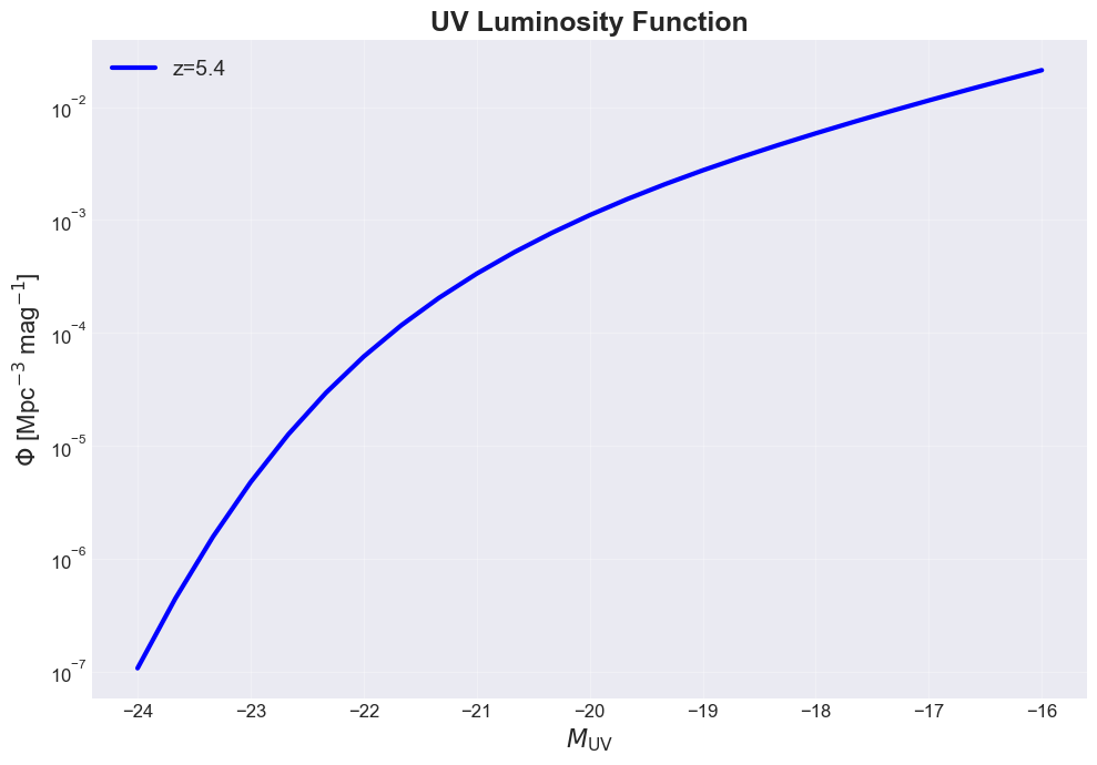
Part 2: UV Luminosity Function

The luminosity function Φ(M_UV) tells us the number density of galaxies as a function of UV magnitude.

# Define magnitude range
MUV = np.linspace(-24, -16, 25)

# Compute luminosity function
print("Computing luminosity function...")
phi = obs.luminosity_function(MUV)

print(f"  Magnitude range: {MUV.min():.1f} to {MUV.max():.1f}")
print(f"  Φ range: {phi.min():.2e} to {phi.max():.2e} Mpc^-3 mag^-1")

Computing luminosity function...
  Magnitude range: -24.0 to -16.0
  Φ range: 1.07e-07 to 2.13e-02 Mpc^-3 mag^-1

# Plot the luminosity function
fig, ax = plt.subplots(figsize=(10, 7))

ax.semilogy(MUV, phi, 'b-', linewidth=3, label=f'z={model.z}')
ax.set_xlabel(r'$M_{\rm UV}$', fontsize=16)
ax.set_ylabel(r'$\Phi$ [Mpc$^{-3}$ mag$^{-1}$]', fontsize=16)
ax.set_title('UV Luminosity Function', fontsize=18, fontweight='bold')
ax.legend(fontsize=14)
ax.grid(True, alpha=0.3)
ax.tick_params(labelsize=12)

plt.tight_layout()
plt.show()

Part 3: Galaxy Bias

Galaxy bias b_g quantifies how strongly galaxies cluster compared to the underlying dark matter.

# Compute galaxy bias
print("Computing galaxy bias...")
bias = obs.galaxy_bias(MUV)

print(f"  Bias range: {bias.min():.2f} to {bias.max():.2f}")

Computing galaxy bias...
  Bias range: 2.70 to 9.70

# Plot galaxy bias
fig, ax = plt.subplots(figsize=(10, 7))

ax.plot(MUV, bias, 'r-', linewidth=3, label=f'z={model.z}')
ax.set_xlabel(r'$M_{\rm UV}$', fontsize=16)
ax.set_ylabel('Galaxy Bias $b_g$', fontsize=16)
ax.set_title('Galaxy Clustering Bias', fontsize=18, fontweight='bold')
ax.legend(fontsize=14)
ax.grid(True, alpha=0.3)
ax.tick_params(labelsize=12)

plt.tight_layout()
plt.show()

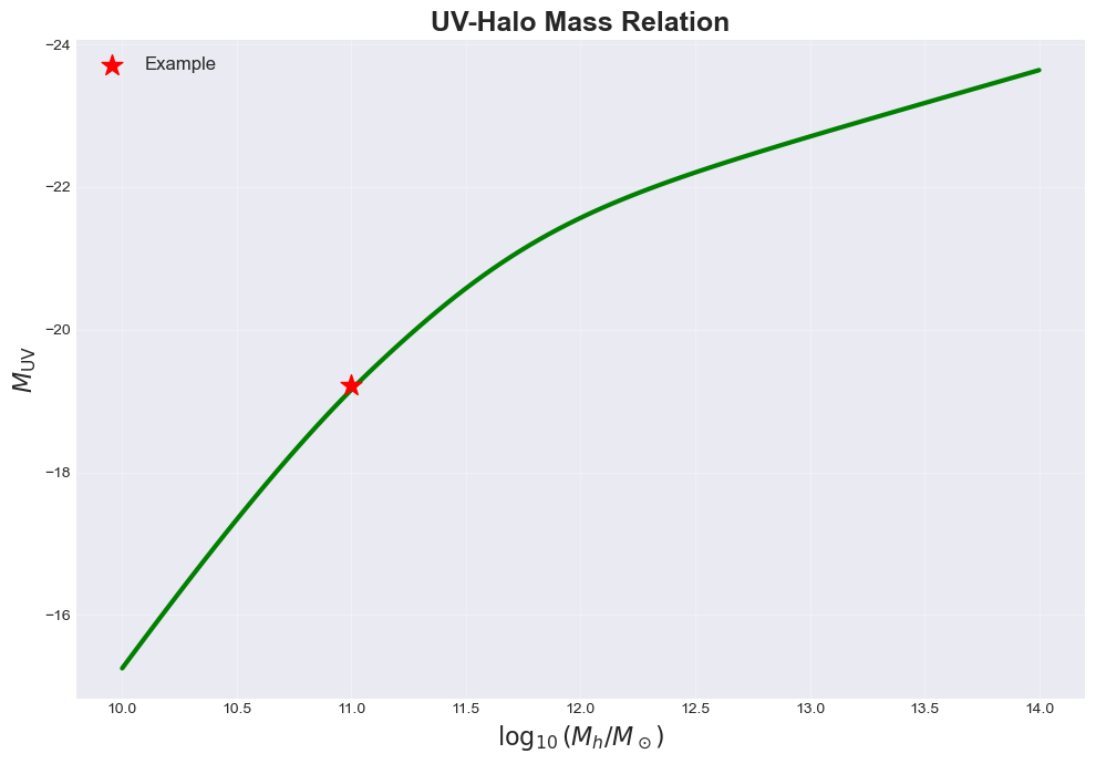
Part 4: UV-Halo Mass Relation

The HODModel inherits all UVHMR methods from the base class. Note that these are not available in the Observables class

# Explore UVHMR for a single halo
Mh_example = 1e11  # M_sun

sfr = model.sfr(Mh_example)
MUV_example = model.MUV(Mh_example)
epsilon = model.star_formation_efficiency(Mh_example)

print(f"Halo mass: {Mh_example:.2e} M_sun")
print(f"  SFR: {sfr} M_sun/yr")
print(f"  M_UV: {MUV_example}")
print(f"  SFE: {epsilon}")

Halo mass: 1.00e+11 M_sun
  SFR: [4.34936672] M_sun/yr
  M_UV: [-19.21614823]
  SFE: [0.12070767]

# Plot UVHMR
Mh_array = np.logspace(10, 14, 100)
MUV_array = model.MUV(Mh_array)

fig, ax = plt.subplots(figsize=(10, 7))

ax.plot(np.log10(Mh_array), MUV_array, 'g-', linewidth=3)
ax.scatter(np.log10(Mh_example), MUV_example, s=200, c='red',
           marker='*', zorder=5, label=f'Example')

ax.set_xlabel(r'$\log_{10}(M_h / M_\odot)$', fontsize=16)
ax.set_ylabel(r'$M_{\rm UV}$', fontsize=16)
ax.set_title('UV-Halo Mass Relation', fontsize=18, fontweight='bold')
ax.invert_yaxis()
ax.legend(fontsize=12)
ax.grid(True, alpha=0.3)

plt.tight_layout()
plt.show()

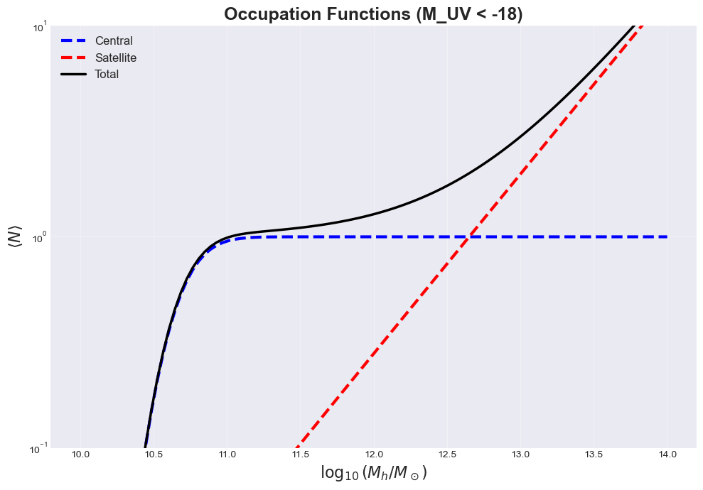
Part 5: Halo Occupation Distribution

MUV_thresh = -18
Mh_range = np.logspace(10, 14, 100)

N_cen = model.Ncen(Mh_range, MUV_thresh)
N_sat = model.Nsat(Mh_range, MUV_thresh)
N_tot = model.Ngal(Mh_range, MUV_thresh)

print(f"For M_UV < {MUV_thresh}:")
print(f"  Peak N_cen: {N_cen.max():.3f}")
print(f"  Max N_sat: {N_sat.max():.2f}")

For M_UV < -18:
  Peak N_cen: 1.000
  Max N_sat: 14.04

fig, ax = plt.subplots(figsize=(10, 7))

ax.plot(np.log10(Mh_range), N_cen, 'b--', linewidth=3, label='Central')
ax.plot(np.log10(Mh_range), N_sat, 'r--', linewidth=3, label='Satellite')
ax.plot(np.log10(Mh_range), N_tot, 'k-', linewidth=2.5, label='Total')

ax.set_ylim(0.1,10)
ax.set_yscale('log')
ax.set_xlabel(r'$\log_{10}(M_h / M_\odot)$', fontsize=16)
ax.set_ylabel(r'$\langle N \rangle$', fontsize=16)
ax.set_title(f'Occupation Functions (M_UV < {MUV_thresh})', fontsize=18, fontweight='bold')
ax.legend(fontsize=12)
ax.grid(True, alpha=0.3)

plt.tight_layout()
plt.show()

Part 6: Mean Properties

thresholds = [-21, -20, -19, -18, -17]

print("Mean Properties by Brightness Threshold:")
print("="*60)

for thresh in thresholds:
    mean_mass = obs.mean_halo_mass(thresh)
    mean_b = obs.mean_bias(thresh)

    print(f"\nM_UV < {thresh}:")
    print(f"  Mean halo mass: {10**mean_mass:.2e} M_sun")
    print(f"  Mean bias: {mean_b:.2f}")

Mean Properties by Brightness Threshold:
============================================================

M_UV < -21:
  Mean halo mass: 4.74e+11 M_sun
  Mean bias: 6.08

M_UV < -20:
  Mean halo mass: 2.67e+11 M_sun
  Mean bias: 5.17

M_UV < -19:
  Mean halo mass: 1.56e+11 M_sun
  Mean bias: 4.48

M_UV < -18:
  Mean halo mass: 9.53e+10 M_sun
  Mean bias: 3.95

M_UV < -17:
  Mean halo mass: 5.99e+10 M_sun
  Mean bias: 3.52

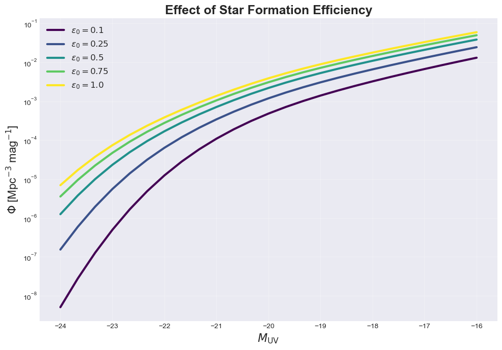
Part 7: Parameter Exploration

All observable methods on Observables accept inline **params keyword arguments to update the model and recompute in a single call — no need to manually call update_parameters() first. This is particularly useful for parameter sweeps and MCMC fitting.

# Create an Observables object — the entry point for all computed quantities
model_var = HODModel(z=6)
obs_var = Observables(model_var)

eps0_values = [0.1, 0.25, 0.5, 0.75, 1.0]
colors = plt.cm.viridis(np.linspace(0, 1, len(eps0_values)))

fig, ax = plt.subplots(figsize=(10, 7))

for eps0, color in zip(eps0_values, colors):
    # Pass eps0 directly — the model is updated internally
    phi_var = obs_var.luminosity_function(MUV, eps0=eps0)
    ax.semilogy(MUV, phi_var, linewidth=3, color=color,
                label=f'$\epsilon_0={eps0}$')

ax.set_xlabel(r'$M_{\rm UV}$', fontsize=16)
ax.set_ylabel(r'$\Phi$ [Mpc$^{-3}$ mag$^{-1}$]', fontsize=16)
ax.set_title('Effect of Star Formation Efficiency', fontsize=18, fontweight='bold')
ax.legend(fontsize=12)
ax.grid(True, alpha=0.3)

plt.tight_layout()
plt.show()

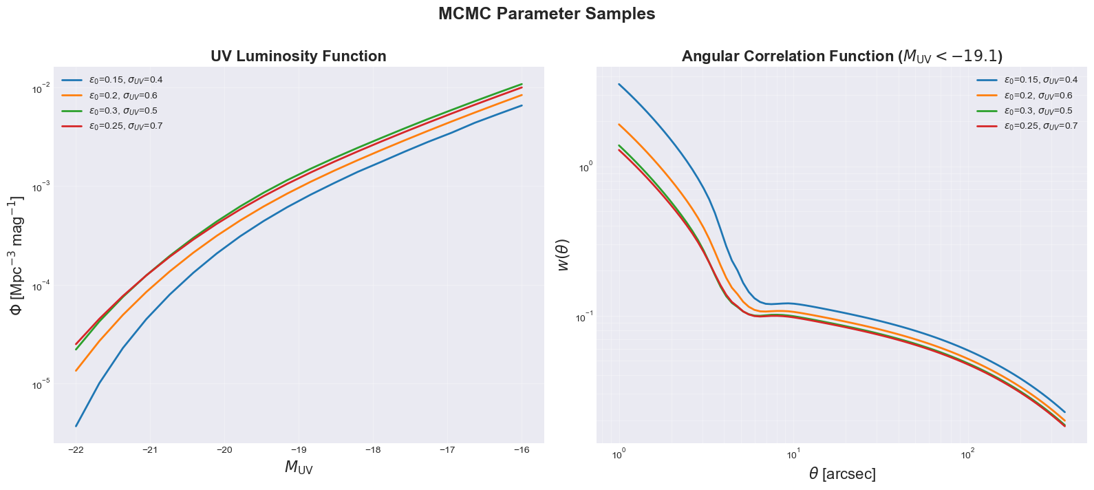
Part 8: Efficient MCMC Fitting with Observables

The Observables class is designed for efficient parameter inference. All observable methods accept **params to update the underlying model in-place before computing, avoiding object re-creation in tight loops.

For correlation functions specifically, use the initialize_correlation_model() / update_correlation_model() pattern which leverages halomod’s internal caching.

# Simulate an MCMC-like loop computing multiple observables per step
obs_mcmc = Observables(HODModel(z=6.0))
MUV_grid = np.linspace(-22, -16, 20)

# Fake MCMC samples: (eps0, sigma_UV)
mcmc_samples = [(0.15, 0.4), (0.20, 0.6), (0.30, 0.5), (0.25, 0.7)]

# --- Initialize the correlation function model once (expensive) ---
result0 = obs_mcmc.initialize_correlation_model(
    MUV_thresh1=-19.1, correlation_type='angular',
    theta_min=1.0, theta_max=360.0, theta_num=80
)

results = []
for eps0, sigma_UV in mcmc_samples:
    # Luminosity function with inline parameter updates
    phi  = obs_mcmc.luminosity_function(MUV_grid, eps0=eps0, sigma_UV=sigma_UV)
    mh   = obs_mcmc.mean_halo_mass(-19.0, eps0=eps0, sigma_UV=sigma_UV)
    ngal = obs_mcmc.number_density(-19.0, eps0=eps0, sigma_UV=sigma_UV)

    # Correlation function via the efficient update path
    cf = obs_mcmc.update_correlation_model(eps0=eps0, sigma_UV=sigma_UV)

    results.append({
        'eps0': eps0, 'sigma_UV': sigma_UV,
        'phi': phi, 'log_Mh': mh, 'n_gal': ngal,
        'theta': cf['separation'], 'w_theta': cf['correlation'],
    })
    print(f"eps0={eps0:.2f}, sigma_UV={sigma_UV:.1f}  →  "
          f"<log Mh>={mh:.2f}, n_gal={ngal:.2e} Mpc^-3")

# --- Plot ---
fig, (ax1, ax2) = plt.subplots(1, 2, figsize=(16, 7))

for r in results:
    label = f"$\\epsilon_0$={r['eps0']}, $\\sigma_{{UV}}$={r['sigma_UV']}"

    # Left: luminosity function
    ax1.semilogy(MUV_grid, r['phi'], linewidth=2, label=label)

    # Right: angular correlation function
    ax2.loglog(r['theta'], r['w_theta'], linewidth=2, label=label)

ax1.set_xlabel(r'$M_{\rm UV}$', fontsize=16)
ax1.set_ylabel(r'$\Phi$ [Mpc$^{-3}$ mag$^{-1}$]', fontsize=16)
ax1.set_title('UV Luminosity Function', fontsize=16, fontweight='bold')
ax1.legend(fontsize=10)
ax1.grid(True, alpha=0.3)

ax2.set_xlabel(r'$\theta$ [arcsec]', fontsize=16)
ax2.set_ylabel(r'$w(\theta)$', fontsize=16)
ax2.set_title(r'Angular Correlation Function ($M_{\rm UV}<-19.1$)',
              fontsize=16, fontweight='bold')
ax2.legend(fontsize=10)
ax2.grid(True, alpha=0.3, which='both')

plt.suptitle('MCMC Parameter Samples', fontsize=18, fontweight='bold', y=1.01)
plt.tight_layout()
plt.show()

/Users/mshuntov/opt/anaconda3/envs/py311/lib/python3.11/site-packages/hmf/density_field/transfer_models.py:232: UserWarning: 'extrapolate_with_eh' was not set. Defaulting to True, which is different behaviour than versions <=3.4.4. This warning may be removed in v4.0. Silence it by setting extrapolate_with_eh explicitly.
  warnings.warn(
/Users/mshuntov/opt/anaconda3/envs/py311/lib/python3.11/site-packages/halomod/integrate_corr.py:567: UserWarning: Filter function p(x) did not integrate to 1 (0.9544997333075783). Tentatively re-normalising.
  p1 = _check_p(p1, z if p_of_z else x)
/Users/mshuntov/opt/anaconda3/envs/py311/lib/python3.11/site-packages/hmf/_internals/_cache.py:115: UserWarning: Using halofit for tracer stats is only valid up to quasi-linear scales k<~1 (h/Mpc).
  value = f(self)
/Users/mshuntov/opt/anaconda3/envs/py311/lib/python3.11/site-packages/halomod/integrate_corr.py:567: UserWarning: Filter function p(x) did not integrate to 1 (0.9544997333075783). Tentatively re-normalising.
  p1 = _check_p(p1, z if p_of_z else x)

eps0=0.15, sigma_UV=0.4  →  <log Mh>=11.18, n_gal=5.91e-04 Mpc^-3
eps0=0.20, sigma_UV=0.6  →  <log Mh>=11.08, n_gal=8.72e-04 Mpc^-3
eps0=0.30, sigma_UV=0.5  →  <log Mh>=11.02, n_gal=1.22e-03 Mpc^-3
eps0=0.25, sigma_UV=0.7  →  <log Mh>=11.01, n_gal=1.14e-03 Mpc^-3

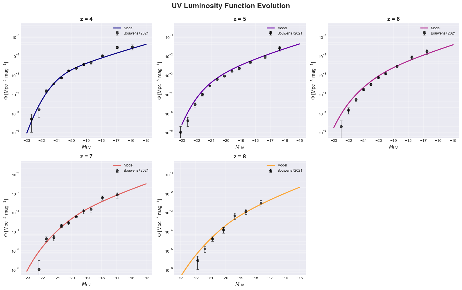
Part 9: Comparison to Observations

Compare model predictions to Bouwens+2021 data.

# Load observational data
from bouwens21_data import bouwens21, redshift_centers

print("Loaded Bouwens+2021 data:")
for key in bouwens21.keys():
    print(f"  {key}: z={redshift_centers[key]}, {len(bouwens21[key]['M_AB'])} points")

Loaded Bouwens+2021 data:
  z4: z=4, 12 points
  z5: z=5, 12 points
  z6: z=6, 10 points
  z7: z=7, 10 points
  z8: z=8, 7 points

# Comparison at different redshifts in 3x3 panels (last panel = all combined)
from halogal.models.parametrization import *
from halogal.config import DEFAULT_REDSHIFT_EVOLUTION

redshift_bins = ['z4', 'z5', 'z6', 'z7', 'z8']
colors = plt.cm.plasma(np.linspace(0, 0.8, len(redshift_bins)))

# Create a single Observables object for all redshifts
obs_compare = Observables(HODModel(z=5.0))

fig, axes = plt.subplots(2, 3, figsize=(16, 10))
axes = axes.flatten()
axes.flatten()[5].axis('off')

for idx, (zbin, color) in enumerate(zip(redshift_bins, colors)):
    ax = axes[idx]
    z_val = redshift_centers[zbin]

    # Get evolved parameters using fitted evolution
    eps0_z = eps0_fz(
        z_val,
        deps_dz=DEFAULT_REDSHIFT_EVOLUTION['d_eps0_dz'],
        eps_off=DEFAULT_REDSHIFT_EVOLUTION['C_eps0'])

    Mc_z = 10**Mc_fz(
        z_val,
        dMc_dz=DEFAULT_REDSHIFT_EVOLUTION['d_logMc_dz'],
        Mc_off=DEFAULT_REDSHIFT_EVOLUTION['C_logMc'])

    a_z = a_fz(
        z_val,
        da_dz=DEFAULT_REDSHIFT_EVOLUTION['d_a_dz'],
        a_off=DEFAULT_REDSHIFT_EVOLUTION['C_a'])

    b_z = b_fz(
        z_val,
        db_dz=DEFAULT_REDSHIFT_EVOLUTION['d_b_dz'],
        b_off=DEFAULT_REDSHIFT_EVOLUTION['C_b'])

    sigmaUV_z = sigma_UV_fz(
        z_val,
        dsigmaUV_dz=DEFAULT_REDSHIFT_EVOLUTION['d_sigmaUV_dz'],
        sigmaUV_off=DEFAULT_REDSHIFT_EVOLUTION['C_sigmaUV'])

    Mcut_z = 10**Mcut_fz(
        z_val,
        dMcut_dz=DEFAULT_REDSHIFT_EVOLUTION['d_Mcut_dz'],
        Mcut_off=DEFAULT_REDSHIFT_EVOLUTION['C_Mcut'])

    Msat_z = 10**Msat_fz(
        z_val,
        dMsat_dz=DEFAULT_REDSHIFT_EVOLUTION['d_Msat_dz'],
        Msat_off=DEFAULT_REDSHIFT_EVOLUTION['C_Msat'])

    asat_z = asat_fz(
        z_val,
        dasat_dz=DEFAULT_REDSHIFT_EVOLUTION['d_asat_dz'],
        asat_off=DEFAULT_REDSHIFT_EVOLUTION['C_asat'])

    # Compute UVLF with inline parameter updates
    MUV_model = np.linspace(-23, -15, 40)
    phi_model = obs_compare.luminosity_function(
        MUV_model,
        z=z_val, eps0=eps0_z, Mc=Mc_z, a=a_z, b=b_z,
        sigma_UV=sigmaUV_z, Mcut=Mcut_z, Msat=Msat_z, asat=asat_z)

    # Plot model
    ax.semilogy(MUV_model, phi_model, '-', linewidth=2.5, color=color,
                label='Model')

    # Plot observations
    data = bouwens21[zbin]
    ax.errorbar(data['M_AB'], data['Fi_k'], yerr=data['Fi_k_error'],
                fmt='o', color='black', markersize=6, capsize=3,
                alpha=0.7, label='Bouwens+2021')

    # Panel styling
    ax.set_xlabel(r'$M_{\rm UV}$', fontsize=12)
    ax.set_ylabel(r'$\Phi$ [Mpc$^{-3}$ mag$^{-1}$]', fontsize=12)
    ax.set_title(f'z = {z_val}', fontsize=14, fontweight='bold')
    ax.set_ylim(5e-7, 5e-1)
    ax.legend(fontsize=9)
    ax.grid(True, alpha=0.3, which='both')
    ax.tick_params(labelsize=10)


plt.suptitle('UV Luminosity Function Evolution', fontsize=18, fontweight='bold', y=0.995)
plt.tight_layout()
plt.show()